How to Use the Lookup Function in Excel

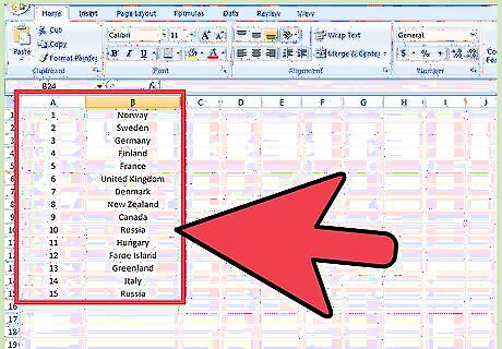
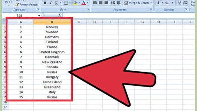
Create a two column list toward the bottom of the page. In this example, one column has numbers and the other has random words.

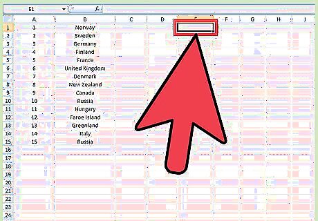
Decide on cell that you would like the user to select from, this is where a drop down list will be.

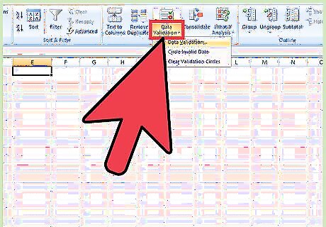
Once you click on the cell, the border should darken, select the DATA tab on the tool bar, then select VALIDATION.

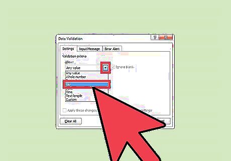
A pop up should appear, in the ALLOW list pick LIST.

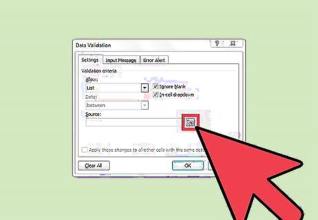
Now to pick your source, in other words your first column, select the button with the red arrow.

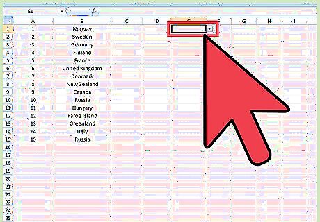
Select the first column of your list and press enter and click OK when the data validation window appears, now you should see a box with an arrow on, if you click on it your list should drop down.

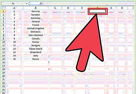
Select another box where you want the other information to show up.

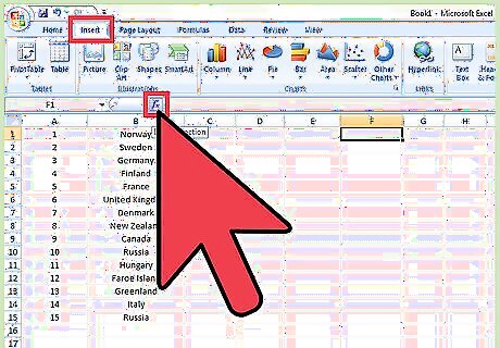
Once you clicked that box, go to the INSERT tab and FUNCTION.

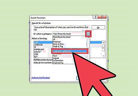
Once the box pops up, select LOOKUP & REFERENCE from the category list.

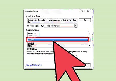
Find LOOKUP in the list and double-click it, another box should appear click OK.

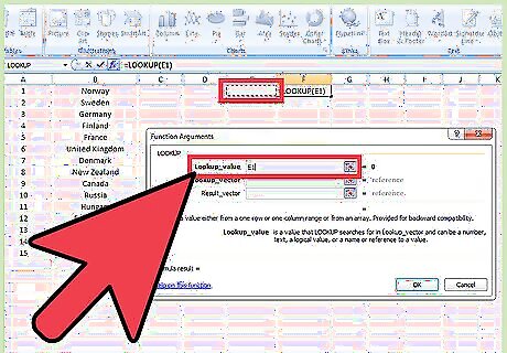
For the lookup_value select the cell with the drop down list.

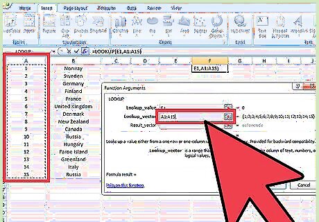
For the Lookup_vector select the first column of your list.

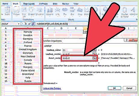
For the Result_vector select the second column.

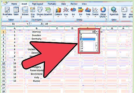
Now whenever you pick something from the drop down list the info should automatically change.