views
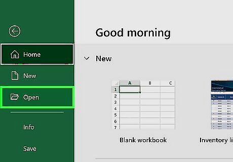
Open a workbook in Microsoft Excel. You can use an existing project or create a new spreadsheet. Make sure you're on the correct worksheet. Microsoft Excel is available on Windows and Mac. You can also use the online web version at https://www.office.com/.
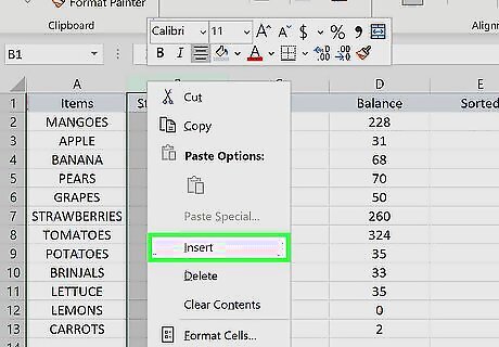
Insert a new column next to the text you want to convert. This will be a temporary column that holds the formula; it can be deleted afterwards. Right-click the column header to the right of where you want to add a new column. Select Insert.
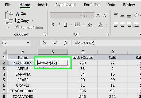
Type =LOWER(cell) into the empty cell. Replace cell with the first cell number of the column you want to convert. This formula will allow you to convert a cell to lowercase letters. For example, to convert cell A2, the formula should look like =LOWER(A2). Alternatively, you can use the =PROPER(cell) formula to convert to the proper case with the initials capitalized, or =UPPER(cell) to convert to uppercase.
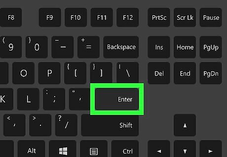
Press ↵ Enter or ⏎ Return on your keyboard. This will process your formula and convert your text in the specified cell to lowercase letters. The converted text will show up in your formula cell here.
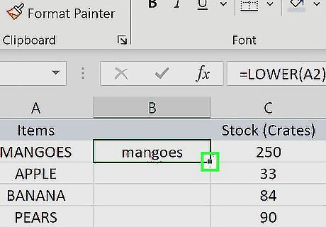
Select the formula cell and double-click the square. This is the small black square at the bottom-right corner of the formula cell. This will fill down the formula in the new column and select the new values.
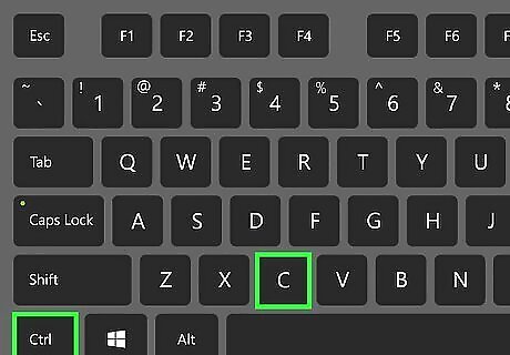
Press Ctrl+C to copy the values. On Mac, this will be CMD + C.
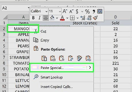
Right-click the first cell of the column you want to convert. In this example, this would be A2. You'll need to paste the converted values to the column.
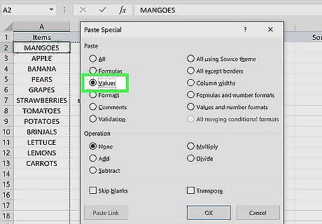
Select Values under "Paste Options". This looks like a clipboard with 123 on it. On some devices, you may need to click Paste, and then Values.
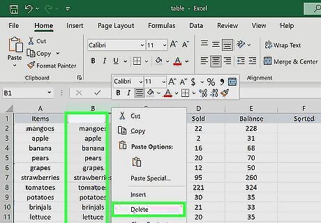
Delete the temporary column. After you paste the new values, you'll no longer need the formulas within the temporary column. Right-click the column header and click Delete.


Comments
0 comment