
views
Standard Deviation and Covariance

Gather stock returns. In order to calculate the correlation coefficient, you will need information on returns (daily price changes) for two stocks over the same period of time. Returns are calculated as the difference between the closing prices of the stock over two days of trading. For example, if a stock closed at $2.00 on Tuesday and $2.04 on Wednesday, this would represent a return of 2 percent. Stock price information can be gathered from market-tracking websites, such as Bloomberg and Yahoo! Finance. Organize your returns as a sequence when you have your data, recording the two stocks in question as stock X and stock Y to simplify your calculations. For example, your data for stock X might be 0.9, 1.3, 1.7, 0.4, 0.7 over five days, while the data for Y is 2.5, 3.5, 3.6, 3.1, 2.3. Correlation coefficients can vary or even switch signs over time (from positive to negative), so the period of time you choose is important. Short-term traders may be fine using 20 or 50 days' worth of data, but longer-term investors will want to use 150 or 250.
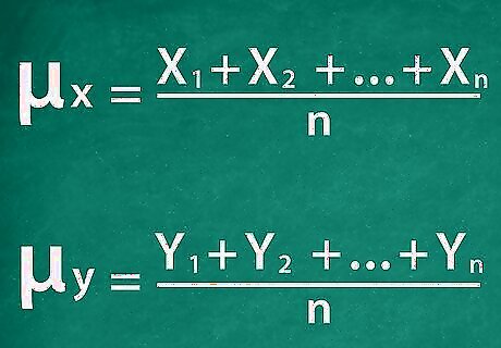
Calculate the mean of each set. Find the average (the mean) of your sets of stock returns by adding each them up and dividing by the number of days in your chosen period (n). The mean will be represented using the Greek letter μ {\displaystyle \mu } \mu , with μ x {\displaystyle \mu _{x}} \mu _{{x}} representing the mean of the returns from stock X and μ y {\displaystyle \mu _{y}} \mu _{{y}} representing the mean of Y's returns. Continuing with the previous example, the number of days, n, would be 5. This means that the mean of X's returns would be μ x = 0.9 + 1.3 + 1.7 + 0.4 + 0.7 5 {\displaystyle \mu _{x}={\frac {0.9+1.3+1.7+0.4+0.7}{5}}} \mu _{{x}}={\frac {0.9+1.3+1.7+0.4+0.7}{5}}, or 1.0. Similarly, Y's returns would average μ y = 2.5 + 3.5 + 3.6 + 3.1 + 2.3 5 {\displaystyle \mu _{y}={\frac {2.5+3.5+3.6+3.1+2.3}{5}}} \mu _{{y}}={\frac {2.5+3.5+3.6+3.1+2.3}{5}}, or 3.0.
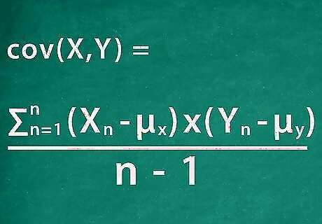
Calculate the covariance. Covariance represents the relationship between two moving variables. If the variable increase or decrease at the same times, they are positively correlated and the covariance is positive. If they move opposite of each other, however, the covariance is negative. Covariance is calculated using the following formula: σ x y = ∑ n = 1 n ( X n − μ x ) × ( Y n − μ y ) n − 1 {\displaystyle \sigma _{xy}={\frac {\sum _{n=1}^{n}(X_{n}-\mu _{x})\times (Y_{n}-\mu _{y})}{n-1}}} \sigma _{{xy}}={\frac {\sum _{{n=1}}^{{n}}(X_{{n}}-\mu _{{x}})\times (Y_{{n}}-\mu _{{y}})}{n-1}}. In the formula, X n {\displaystyle X_{n}} X_{{n}} and Y n {\displaystyle Y_{n}} Y_{{n}} represent the stock's return on each day in the period. The idea is to sum up the product of the differences between the stock return and mean return for each day. For example, the part of the covariance formula for first day would be calculated as: ( 0.9 − 1.0 ) × ( 2.5 − 3.0 ) {\displaystyle (0.9-1.0)\times (2.5-3.0)} (0.9-1.0)\times (2.5-3.0). This would then be added to the result for the other four days then divided by 4 (5-1). This solves to 0.77 4 {\displaystyle {\frac {0.77}{4}}} {\frac {0.77}{4}}, which is 0.1925. The covariance between returns on stock X and Y is 0.1925.
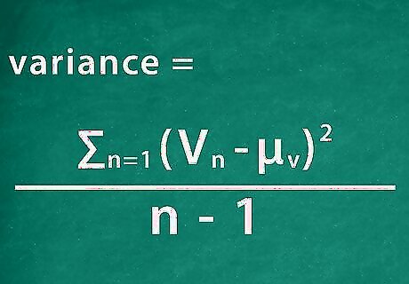
Calculate the variance of each stock. Variance is similar to covariance, but is calculated separately for each variable or, in this case, set of stock returns. It represents how strongly a variable moves above or below its mean over the period. The calculation is also quite similar to that for covariance, but it replace the product of the two variables' differences with a square of the same variable's difference from the mean. Specifically, the equation is: ∑ n = 1 n ( V n − μ V ) 2 n − 1 {\displaystyle {\frac {\sum _{n=1}^{n}(V_{n}-\mu _{V})^{2}}{n-1}}} {\frac {\sum _{{n=1}}^{{n}}(V_{{n}}-\mu _{{V}})^{{2}}}{n-1}} where V represents the variable in question (either X or Y). This means that the part of the variance equation for first day of returns for stock X would be calculated as ( 0.9 − 1.0 ) 2 {\displaystyle (0.9-1.0)^{2}} (0.9-1.0)^{{2}}, which would solve to 0.01. Continue this for each day of X, adding them up as you go along. Then, divide by n − 1 {\displaystyle n-1} n-1 to get your answer. For the example, the top calculation would be 0.832, so the variable is that divided by 4, or 0.208. This means that the variance of X's returns, σ x 2 {\displaystyle \sigma _{x}^{2}} \sigma _{{x}}^{{2}}, is 0.208. Following the same process with Y yields σ y 2 = 0.272 {\displaystyle \sigma _{y}^{2}=0.272} \sigma _{{y}}^{{2}}=0.272.
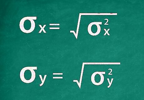
Find the standard deviation. The standard deviation, σ {\displaystyle \sigma } \sigma , is the square root of the variance. Simply take the square roots of σ x 2 {\displaystyle \sigma _{x}^{2}} \sigma _{{x}}^{{2}} and σ y 2 {\displaystyle \sigma _{y}^{2}} \sigma _{{y}}^{{2}} to get their respective standard deviations. After calculations, the results are σ x = 0.456 {\displaystyle \sigma _{x}=0.456} \sigma _{{x}}=0.456 σ y = 0.522 {\displaystyle \sigma _{y}=0.522} \sigma _{{y}}=0.522. Note that these calculations have been rounded to three decimal places to ease later calculations. Keeping more decimal places in your calculations will make them more accurate.
Correlation Coefficient
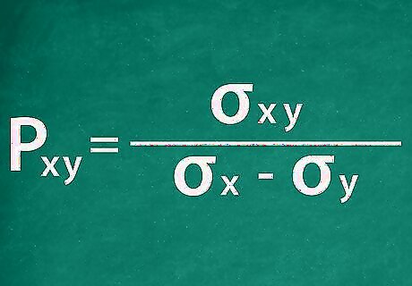
Set up your correlation coefficient equation. The Pearson correlation coefficient is luckily a good amount simpler to calculate than its constituent parts, the covariance and standard deviations. The correlation coefficient of X and Y, ρ x y {\displaystyle \rho _{xy}} \rho _{{xy}}, is calculated as σ x y σ x × σ y {\displaystyle {\frac {\sigma _{xy}}{\sigma {x}\times \sigma {y}}}} {\frac {\sigma _{{xy}}}{\sigma {x}\times \sigma {y}}}. In simple terms, it is the covariance of X and Y divided by the product of their standard deviations. For the example stocks, your equation would be set up as ρ x y = 0.1925 0.456 × 0.522 {\displaystyle \rho _{xy}={\frac {0.1925}{0.456\times 0.522}}} \rho _{{xy}}={\frac {0.1925}{0.456\times 0.522}}
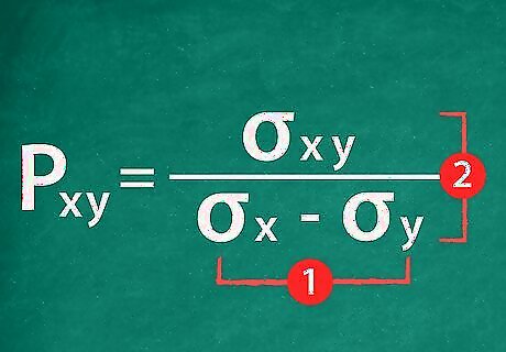
Solve for the correlation coefficient. Start by simplifying the bottom of the equation by multiplying the two standard deviations. Then, divide the covariance on the top by your result. The solution is your correlation coefficient. The coefficient is represented as a decimal between -1 and 1, rather than as a percentage. Continuing with the example, the equation solves to ρ x y = 0.809 {\displaystyle \rho _{xy}=0.809} \rho _{{xy}}=0.809. So, the correlation coefficient between returns on stocks X and Y is 0.809. Note that this result has been rounded to three decimal places.
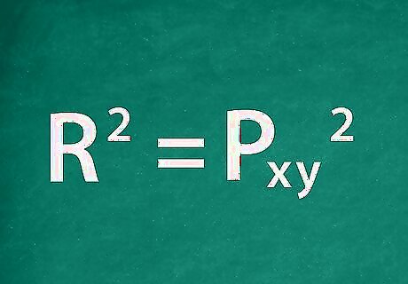
Calculate R-squared. The square of the correlation coefficient, called R-squared, is also used to measure how closely the returns are linearly related. In simpler terms, it represents how much of the movement in one variable is caused by the other. It does, however, specify which variable acts upon the other (if X causes Y to move or if Y causes X to). Calculate R-squared by squaring your result for the correlation coefficient. For example, the R-squared value for the example correlation coefficient would be ρ x y 2 = 0.809 2 = 0.654. {\displaystyle \rho _{xy}^{2}=0.809^{2}=0.654.} \rho _{{xy}}^{{2}}=0.809^{{2}}=0.654.
Correlation Coefficient Uses
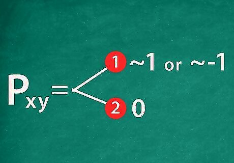
Understand your correlation coefficient result. The correlation coefficient can be understood as an indicator of two things. The first is whether or not the two variables in question typically move in the same direction at the same time. If they do, the correlation coefficient is positive. If not, it is negative. The second thing the correlation coefficient can tell you is how similar these movements are. A correlation coefficient close of 1 or -1 represents perfect positive correlation or perfect negative correlation, respectively. Correlation coefficients always vary between 1 and -1. A result of 0 indicates that there is no correlation. So, for example, the example result of 0.809 from the other part of this article would mean that stocks X and Y are highly correlated. The two securities experience price movements in the same direction and usually in roughly the same magnitude.

Reduce risk in your portfolio. The primary use of stock correlation coefficients is in the preparation of balanced securities portfolios. Stocks or other assets within a portfolio can be assessed against others in the same portfolio to determine the correlation coefficient between them. The goal is to place stocks with low or negative correlations in the same portfolio. Thus, when the price of the first stock moves, the second will likely move oppositely or independently of the first. The result of these actions is effective portfolio diversification. This practice reduces "unsystematic risk," which is risk inherent to individual securities.

Expand your analysis to other assets. The correlation coefficient is also frequently used to assess relationships between other data sets, such as mutual fund returns, Exchange Traded Fund (ETF) returns, and market indexes. Correlations coefficients can be calculated between these data sets and stock returns to diversify a portfolio or to figure out how a stock's price moves in relation to other market shifts. This can be useful for predicting the change in a stock's price that would occur in the event of another change in the market. For example, the stock price of a gold mining company might be positively related to the price of gold (with a high, positive correlation coefficient). If the price of gold is expected to increase, an investor would have reason to believe that the price of the company's stock will as well.
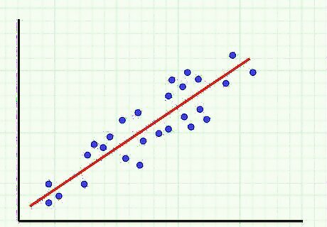
Plot the pairs of stock return data to obtain a 'scatter plot'. You can use a spreadsheet program to plot the dates and returns of your stocks. This makes it easier to note the properties of the data. Also, using spreadsheet software, you can plot a best fit line. The best fit line to the data is called the regression line. On Excel, you can add this line by clicking "Chart" and then "Add Trendline." The program will then calculate a trend line based on your data. The correlation coefficient is a measure of how closely the two stock returns fit the regression line. That is, how closely the return values satisfy a linear relation such as Y = βX + α for some constants α and β.


Comments
0 comment