How to Calculate Covariance

Calculating Covariance by Hand with the Standard Formula

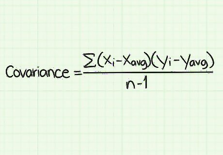
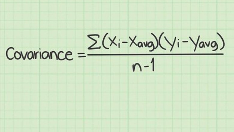
Learn the standard covariance formula and its parts. The standard formula for calculating covariance is Σ ( x i − x avg ) ( y i − y avg ) / ( n − 1 ) {\displaystyle \Sigma (x_{i}-x_{\text{avg}})(y_{i}-y_{\text{avg}})/(n-1)} \Sigma (x_{i}-x_{{\text{avg}}})(y_{i}-y_{{\text{avg}}})/(n-1). To use this formula, you need to understand the meaning of the variables and symbols: Σ {\displaystyle \Sigma } \Sigma - This symbol is the Greek letter “sigma.” In math functions it means to add up a series of whatever follows it. In this formula, the Σ sign means that you will calculate the values that follow in the numerator of the fraction, and add them all together, before dividing by the denominator. x i {\displaystyle x_{i}} x_{i} - This variable is read as “x sub i.” The i subscript represents a counter. It means that you will perform the calculation for each value of x that you have in your data set. x a v g {\displaystyle x_{avg}} x_{{avg}} - The “avg” indicates that x(avg) is the average value of all of your x data points. The average is sometimes also written as an x with a short horizontal line drawn over it. In that style, the variable is read as “x-bar,” but it still means the average of the data set. y i {\displaystyle y_{i}} y_{i} - This variable is read as “y sub i.” The i subscript represents a counter. It means that you will perform the calculation for each value of y that you have in your data set. y a v g {\displaystyle y_{avg}} y_{{avg}} - The “avg” indicates that y(avg) is the average value of all of your y data points. The average is sometimes also written as a y with a short horizontal line drawn over it. In that style, the variable is read as “y-bar,” but it still means the average of the data set. n {\displaystyle n} n - This variable represents the number of items in your data set. Remember that for a covariance problem, a single “item” is comprised of both an x-value and a y-value. The value of n is the number of pairs of data points, not individual numbers.

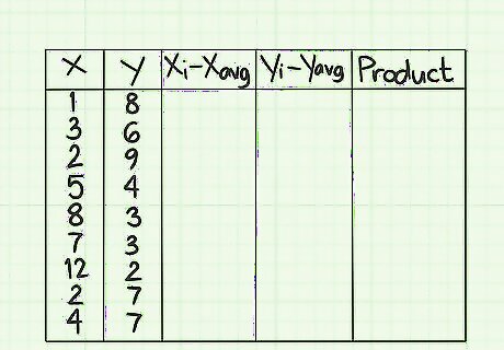
Set up your data table. Before you begin working, it is helpful to collect your data. You should make a table that consists of five columns. You should label each column as follows: x {\displaystyle x} x - fill this column with the values of your x-data points. y {\displaystyle y} y - fill this column with the values of your y-data points. Be careful to align the y-values with the corresponding x-values. In a covariance problem, the order of the data points and the pairings of x and y are important. ( x i − x avg ) {\displaystyle (x_{i}-x_{\text{avg}})} (x_{i}-x_{{\text{avg}}}) - Leave this column blank in the beginning. You will fill it with data after you calculate the average of the x-data points. ( y i − y avg ) {\displaystyle (y_{i}-y_{\text{avg}})} (y_{i}-y_{{\text{avg}}}) - Leave this column blank in the beginning. You will fill it with data after you calculate the average of the y-data points. Product {\displaystyle {\text{Product}}} {\text{Product}} - Leave this final column blank as well. You will fill it as you go along.

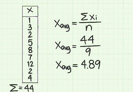
Calculate the average of the x-data points. This sample data set contains 9 numbers. To find the average, add them together and divide the sum by 9. This gives you the result of 1+3+2+5+8+7+12+2+4=44. When you divide by 9, the average is 4.89. This is the value that you will use as x(avg) for the coming calculations.

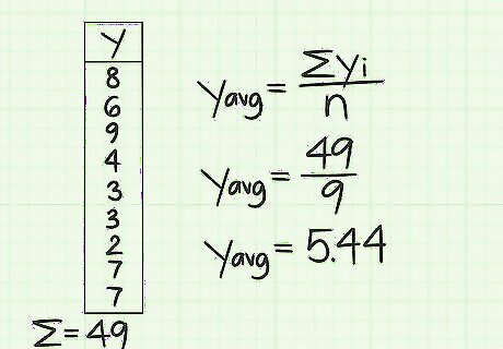
Calculate the average of the y-data points. Similarly, the y-column should consist of 9 data points that coincide with the x-data points. Find the average of these. For this sample data set, this will be 8+6+9+4+3+3+2+7+7=49. Divide this sum by 9 to get an average of 5.44. You will use 5.44 as the value of y(avg) for the coming calculations.

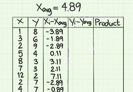
Calculate the ( x i − x avg ) {\displaystyle (x_{i}-x_{\text{avg}})} (x_{i}-x_{{\text{avg}}}) values. For each item in the x column, you need to find the difference between that number and the average value. For this sample problem, this means subtracting 4.89 from each x-data point. If the original data point is less than the average, then your result will be negative. If the original data point is greater than the average, then your result will be positive. Make sure that you keep track of the negative signs. For example, the first data point in the x column is 1. The value to enter on the first line of the ( x i − x avg ) {\displaystyle (x_{i}-x_{\text{avg}})} (x_{i}-x_{{\text{avg}}}) column is 1-4.89, which is -3.89. Repeat the process for each data point. Therefore, the second line will be 3-4.89, which is -1.89. The third line will be 2-4.89, or -2.89. Continue the process for all the data points. The nine numbers in this column should be -3.89, -1.89, -2.89, 0.11, 3.11, 2.11, 7.11, -2.89, -0.89.

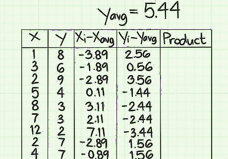
Calculate the ( y i − y avg ) {\displaystyle (y_{i}-y_{\text{avg}})} (y_{i}-y_{{\text{avg}}}) values. In this column, you will perform similar subtractions, using the y-data points and the y average. If the original data point is less than the average, then your result will be negative. If the original data point is greater than the average, then your result will be positive. Make sure that you keep track of the negative signs. For the first line, therefore, your calculation will be 8-5.44, which is 2.56. The second line will be 6-5.44, which is 0.56. Continue these subtractions to the end of the data list. When you finish, the nine values in this column should be 2.56, 0.56, 3.56, -1.44, -2.44, -2.44, -3.44, 1.56, 1.56.

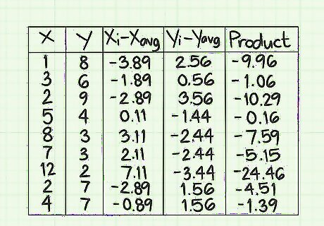
Calculate the products for each data row. You will fill in the rows of the final column by multiplying the numbers that you calculated in the two previous columns of ( x i − x avg ) {\displaystyle (x_{i}-x_{\text{avg}})} (x_{i}-x_{{\text{avg}}}) and ( y i − y avg ) {\displaystyle (y_{i}-y_{\text{avg}})} (y_{i}-y_{{\text{avg}}}). Be careful to work row by row, and multiply the two numbers for the corresponding data points. Keep track of any negative signs as you go. On the first row of this data sample, the ( x i − x avg ) {\displaystyle (x_{i}-x_{\text{avg}})} (x_{i}-x_{{\text{avg}}}) that you calculated is -3.89, and the ( y i − y avg ) {\displaystyle (y_{i}-y_{\text{avg}})} (y_{i}-y_{{\text{avg}}}) value is 2.56. The product of these two numbers is -3.89*2.56=-9.96. For the second row, you will multiply the two numbers -1.88*0.56=-1.06. Continue multiplying row by row to the end of the data set. When you finish, the nine values in this column should be -9.96, -1.06, -10.29, -0.16, -7.59, -5.15, -24.46, -4.51, -1.39.

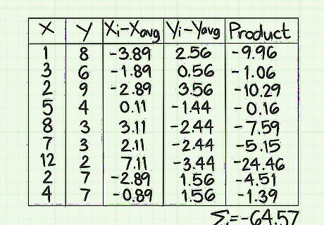
Find the sum of the values in the last column. This is where the Σ symbol comes into play. After conducting all the calculations that you have done so far, you will add the results. For this sample data set, you should have nine values in the final column. Add those nine numbers together. Pay careful attention to whether each number is positive or negative. For this sample data set, the sum should be -64.57. Write this total in the space at the bottom of the column. This represents the value of the numerator of the standard covariance formula.

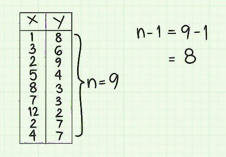
Calculate the denominator for the covariance formula. The numerator for the standard covariance formula is the value that you have just completed calculating. The denominator is represented by (n-1), which is just one less than the number of data pairs in your data set. For this sample problem, there are nine data pairs, so n is 9. The value of (n-1), therefore, is 8.

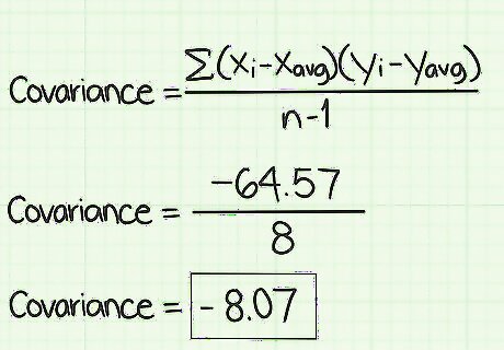
Divide the numerator by the denominator. The final step in calculating the covariance is to divide your numerator, Σ ( x i − x avg ) ( y i − y avg ) {\displaystyle \Sigma (x_{i}-x_{\text{avg}})(y_{i}-y_{\text{avg}})} \Sigma (x_{i}-x_{{\text{avg}}})(y_{i}-y_{{\text{avg}}}) by your denominator, ( n − 1 ) {\displaystyle (n-1)} (n-1). The quotient is the covariance of your data. For this sample data set, this calculation is -64.57/8, which gives the result of -8.07.

Using an Excel Spreadsheet to Calculate Covariance

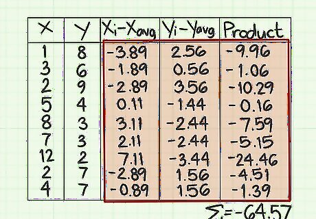
Notice the repetitive calculations. Covariance is a calculation that you should perform a few times by hand, so you understand the meaning of the result. However, if you are going to be using covariance values routinely in interpreting data, you will want to find a faster and more automated way to get your results. You should notice by now that for our relatively small data set of only nine pairs of data, the calculations included finding two averages, performing eighteen individual subtractions, nine separate multiplications, one addition, and a final division. That is 31 relatively minor calculations in order to find one solution. Along the way, you risk dropping negative signs or copying your results incorrectly, thereby ruining the result.

Create a spreadsheet to calculate covariance. If you are comfortable using Excel (or some other spreadsheet with calculation abilities), you can easily set up a table to find covariance. Label the headings of five columns as for the hand calculations: x, y, (x(i)-x(avg)), (y(i)-y(avg)) and Product. To simplify your labelling, you could call the third column something like “x difference” and the fourth column “y difference,” as long as you remember the meaning of the data. If you begin your table in the top left corner of the spreadsheet, then cell A1 will be the x label, with the other labels going across to cell E1.

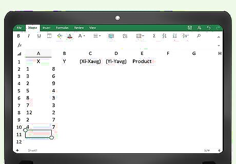
Fill in the data points. Enter your data values in the two columns labelled x and y. Remember that the order of the data points matters, so you need to pair each y with its corresponding x value. Your x values will begin in cell A2 and will continue down for as many data points as you need. Your y values will begin in cell B2 and will continue down for as many data points as you need.

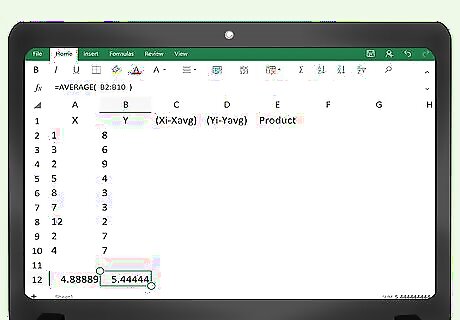
Find the averages of the x and y values. Excel will calculate the averages for you very quickly. In the first vacant cell below each column of data, enter the formula =AVG(A2:A___). Fill in the blank space with the number of the cell that corresponds to your last data point. For example, if you have 100 data points, they will fill in cells A2 through A101, so you will enter =AVG(A2:A101). For the y data, enter the formula =AVG(B2:B101). Remember that you begin a formula in Excel with an = sign.

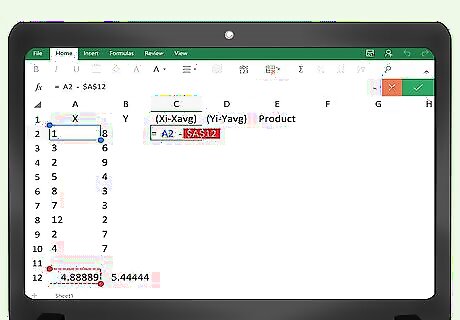
Enter the formula for the (x(i)-x(avg)) column. In cell C2, you will need to enter the formula to calculate the first subtraction. This formula will be =A2-____. You will fill in the blank space with the cell address that contains the average of your x data. For the example of 100 data points, the average would be in cell A103, so your formula will be =A2-A103.

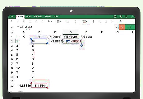
Repeat the formula for the (y(i)-y(avg)) data points. Following the same example, this would go into cell D2. The formula will be =B2-B103.

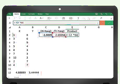
Enter the formula for the “Product” column. In the fifth column, into cell E2, you will need to enter the formula to calculate the product of the two prior cells. This would simply be =C2*D2.

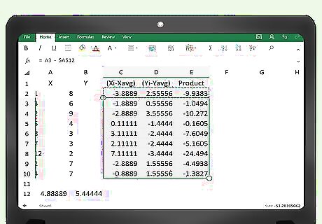
Copy the formulas down to fill the table. So far, you have only programmed the first pair of data points in row 2. Using your mouse, highlight cells C2, D2 and E2. Then position your cursor over the small box in lower right-hand corner until a plus-sign appears. Click your mouse button, hold it down, and drag the mouse downward to expand the highlighted box to fill your entire data table. This step will automatically copy the three formulas from cells C2, D2 and E2 into the whole table. You should see the table automatically fill with all the calculations.

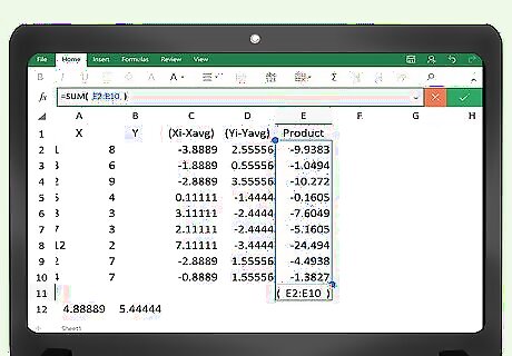
Program the sum of the last column. You need to find the sum of the items in the “Product” column. In the vacant cell immediately under the last data point in that column, enter the formula =sum(E2:E___). Fill in the blank space with the cell address of the last data point. For the example of 100 data points, this formula will go into cell E103. You will enter =sum(E2:E102).

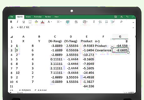
Find the covariance. You can have Excel perform the final calculation for you as well. The last calculation, in cell E103 in our example, represents the numerator of the covariance formula. Immediately below that cell, you can enter the formula =E103/___. Fill in the blank space with the number of data points that you have. In our example, this will be 100. The result will be the covariance of your data.

Using Website Covariance Calculators

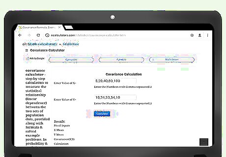
Search the Internet for covariance calculators. Several schools, programming companies or other sources have created websites that will very easily calculate covariance values for you. Using any search engine, enter the search term “covariance calculator.”

Enter your data. Read the instructions on the website carefully to make sure that you enter your data properly. It is important that your data pairs are kept in order, or you will generate an incorrect covariance result. Different websites have different styles for entering your data. For example, at the website http://ncalculators.com/statistics/covariance-calculator.htm, there is a horizontal box for entering x-values and a second horizontal box for entering y-values. You are instructed to enter your terms, separated only by commas. Thus, the x-data set that was calculated earlier in this article would be entered as 1,3,2,5,8,7,12,2,4. The y-data set would be 8,6,9,4,3,3,2,7,7. At another site, https://www.thecalculator.co/math/Covariance-Calculator-705.html, you are prompted to enter your x-data in the first box. Data is entered vertically, with one item per line. Therefore, the entry on this site would look like: 1 3 2 5 8 7 12 2 4

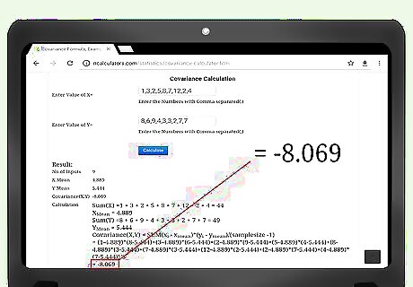
Calculate your results. The attraction of these calculation sites is that after you enter your data, you generally need only to click on the button that says “Calculate,” and the results will appear automatically. Most sites will provide you with the intermediate calculations of the x(avg), y(avg), and n.

Interpreting the Covariance Results

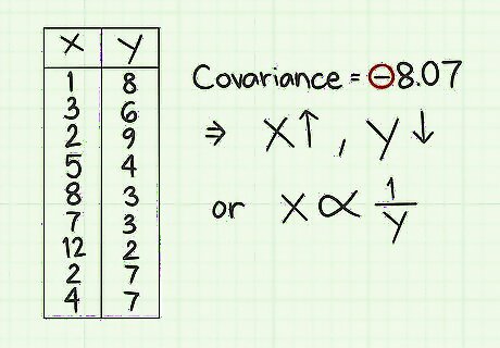
Look for a positive or negative relationship. The covariance is a single statistical figure that represents how one data set relates to another. In the example mentioned in the introduction, height and weight are being measured. You would expect that as individuals grow taller, their weight would also increase, leading to a positive covariance figure. As another example, suppose data is collected representing the number of hours someone practices golf and the score he or she may earn. In this case, you would expect a negative covariance, which means that as the number of practice hours increases, the golf score will decrease. (In golf, a lower score is better.) Consider the sample data set that was calculated above. The resulting covariance is -8.07. The negative sign here means that as the x-values increase, the y-values will tend to decrease. In fact, you can see that this is true by looking at a few of the values. For example, the x-values of 1 and 2 correspond to y-values of 7, 8 and 9. The x-values of 8 and 12 are paired respectively with y-values of 3 and 2.

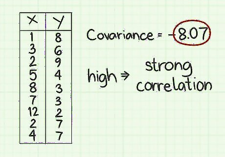
Interpret the magnitude of the covariance. If the number of the covariance score is large, either a large positive number or a large negative number, then you can interpret this as meaning that the two data elements are very strongly connected, either in a positive or negative way. For the sample data set, the covariance of -8.07 is fairly large. Notice that the data values range from 1 through 12, so 8 is a pretty high number. This indicates a strong connection between the x and y data sets.

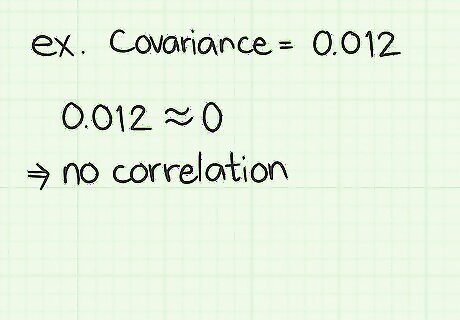
Understand a lack of relationship. If you wind up with a covariance equal to or very near 0, you can conclude that the data points are relatively unrelated. That is, an increase in one value may or may not lead to an increase in the other. The two terms are almost randomly connected. For example, suppose you are comparing shoes sizes against SAT scores. Because there are so many factors that affect a student’s SAT scores, we would expect a covariance score of near 0. This would indicate almost no connection between the two values.

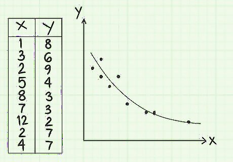
View the relationship graphically. To understand covariance visually, you can plot your data points on the x-y coordinate plane. When you do that, you should see fairly easily that the points, although not in an exactly straight line, tend to form a cluster that approximates a diagonal line from the upper left to the lower right. This is the description of a negative covariance. Also, notice that the covariance value is -8.07. This is a fairly large number compared to the data points. The high number suggests that the covariance is fairly strong, which you can see by the linear appearance of the data points. To review plotting points on the coordinate plane, see Graph Points on the Coordinate Plane.