Calculate Interest Payments on a Loan with the IPMT Function

Glowfly

Editor

posted on 13 years ago — updated on 1 second ago

31
views

This wikiHow teaches you how to create an interest payment calculator in Microsoft Excel. To calculate payments, you'll just need the principal amount, interest rate, and number of payments remaining. You can then use the IPMT function to determine how much you'll have to pay in interest in each period. You can calculate interest payments in Excel on a Windows PC or a Mac.

Things You Should Know

Create row headers for Principal, Interest, Periods, and Payment.
Fill out the principal amount, interest rate, and the number of payment periods.
In the Payment row, use the formula =IPMT(B2, 1, B3, B1) to calculate the interest payment.

Open a Blank Workbook. Launch Excel, then click Blank workbook to get started. Skip this step on Mac.

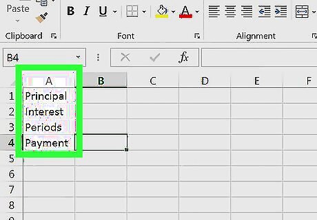
Set up your rows. Enter your payment headings in each of the following cells: Cell A1 - Type in Principal Cell A2 - Type in Interest Cell A3 - Type in Periods Cell A4 - Type in Payment

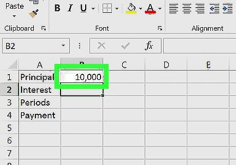
Enter the payment's total value. In cell B1, type in the total amount you owe. For example, if you bought a boat valued at $20,000 for $10,000 down, you would type 10,000 into B1.

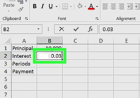
Enter the current interest rate. In cell B2, type in the percentage of the interest that you have to pay each period. For example, if your interest rate is three percent, you would type 0.03 into B2.

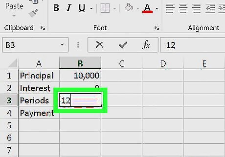
Enter the number of payments you have left. This goes in cell B3. If you're on a 12-month plan, for example, you would type 12 into cell B3.

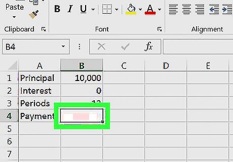
Select cell B4. Simply click B4 to select it. This is where you'll enter the formula to calculate your interest payment.

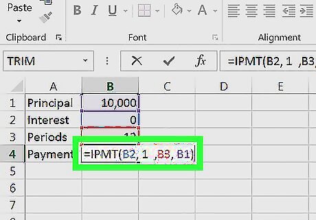
Enter the interest payment formula. Type =IPMT(B2, 1, B3, B1) into cell B4 and press ↵ Enter. Doing so will calculate the amount that you'll have to pay in interest for each period. This doesn't give you the compounded interest, which generally gets lower as the amount you pay decreases. You can see the compounded interest by subtracting a period's worth of payment from the principal and then recalculating cell B4.